About BAMT algorithms
Web-BAMT is a web service that allows you to train Bayesian networks on demonstration examples on data of various nature.
Introduction to Bayesian networks
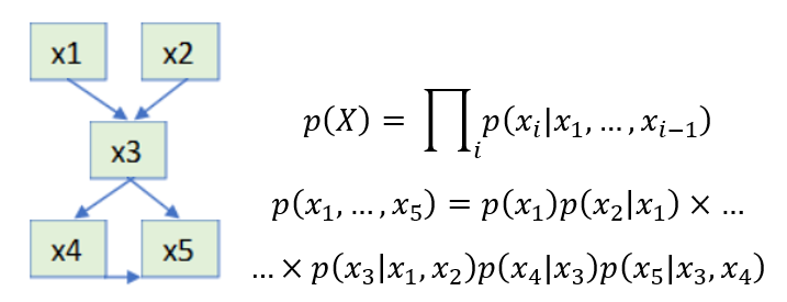
A Bayesian network is a pair of directed acyclic graph (DAG) describing the dependencies of characteristics and some factorization of the joint distribution of characteristics in the product of conditional, generated by these dependencies. Below is an example of a Bayesian network and how a multivariate distribution is factorized according to the structure of the Bayesian network
The task of training a Bayesian network is thus split into two subtasks:
Finding the structure of the Bayesian network.
Parametric learning of the Bayesian network or, in other words, selection of marginal and conditional distributions that describe the conditional ones accurately enough.
Structural learning algorithms
Often the task of constructing a network is reduced to optimization:
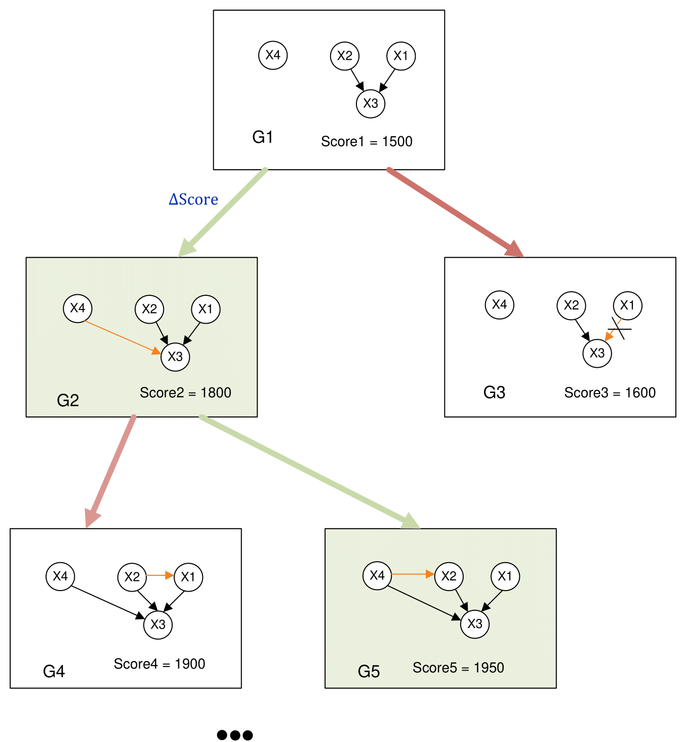
In the DAG space, score functions are introduced that evaluate how well the graph describes the dependencies between features. Web BAMT uses the Hill-Climbing algorithm to search in this space. Steps of Hill-Climbing algorithm:
Initialized by a graph without edges;
For each pair of nodes, an edge is added, removed or the direction is changed;
The score-function value is counted after the selected action on the pair;
If the value of score-function is better than that of the previous iteration, the result is memorized;
Stops when the value changes less than the threshold value.
The following score functions from BAMT package are included in Web BAMT: K2, BIC (Bayesian Information Criterion), MI (Mutual Information).
The above approach to structure search allows to introduce elements of expert control by narrowing the search area to structures that include expert-specified edges or fixed root nodes describing key and basic features. Also, our web service allows you to train connections from continuous to discrete nodes, in this case modeling distributions using classification models (for this you need to set the Logit parameter to True).
Parametric learning algorithms
Parametric learning of distributions is performed by the method of likelihood maximization in a fixed class of distributions.
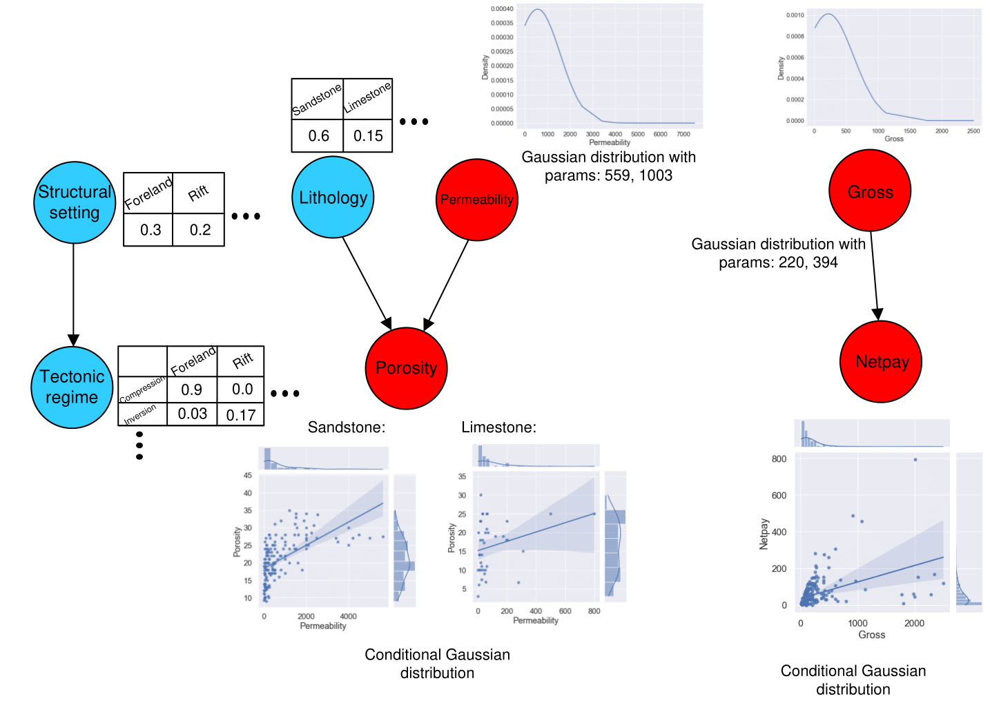
In classical Bayesian networks, at the nodes of a Bayesian network, distributions are represented either using conditional probability tables (for discrete nodes) or using Gaussian distributions and linear regressions (for continuous nodes). However, such a classical approach to modeling conditional distributions may not always be effective since the data is not always modeled by linear regressions. That is why, within the framework of this web service, the ability to work with composite Bayesian networks was added.
Parametric learning algorithms for composite Bayesian networks
The core of the representation of Bayesian networks is a directed acyclic graph,
however, in the composite setting, this core is extended by two types of vertices, namely
G={V,M,E} where G is the structure of the composite Bayesian network, V is a set
of variable nodes within which a probability distribution is modeled, M is a set of
model nodes that are machine learning models and link variable nodes, E is a set of
directed edges. Therefore, for example, if two variable nodes are continuous, then they
can be connected by any machine learning model that can solve the regression problem.
Then the parameters of the conditional continuous distribution for the connection of nodes
X and Y of the form X → m → Y will be calculated as follows:
where μ, var is the mean and variance of the conditional distribution, m is the machine learning model node that links the variable nodes X and Y.
Therefore, as part of working with the web service, the user can choose a machine learning model for both continuous nodes and discrete ones to model conditional distributions in the nodes. This approach more accurately reproduces conditional distributions with non-linear dependencies between nodes.
Sampling algorithms
Sampling in Bayesian networks is done top-down according to the topological order. For the root nodes, the parametric model describes the distribution from which the random value is to be obtained. For discrete ones this is a multinomial discrete distribution, for continuous ones it is a Gaussian distribution or a mixture of Gaussian distributions. Once the values for the root vertices are obtained, all the following distributions are conditional on the values in the parent vertices.
For discrete values, these will also be random values obtained according to the table of conditional distributions estimated from the data in the case of discrete parents or obtained from the classification model if at least one parent is continuous. In the continuous case, the distribution parameters for sampling are obtained using gaussian mixture regression (GMR). If the simple option is chosen, such a model will be degenerate and will have only one mixture element.
For composite models, sampling is performed by predicting the conditional mathematical expectation or conditional probabilities from the selected machine learning model.