Examples
Example methodology description
Both examples consider the following combinations of hyperparameters used for Bayesian network learning:
K2 metric;
K2 metric with gaussian mixtures (GMM);
K2 metric with GMM and logit nodes;
K2 with initial structure.
All the examples are executed using cross-validation, the data is preproccesed as follows:
data.dropna(inplace=True)
data.reset_index(inplace=True, drop=True)

encoder = preprocessing.LabelEncoder()
discretizer = preprocessing.KBinsDiscretizer(n_bins=5, encode='ordinal', strategy='quantile')

p = pp.Preprocessor([('encoder', encoder), ('discretizer', discretizer)])

discretized_data, est = p.apply(train)
Geological data example
Data Description
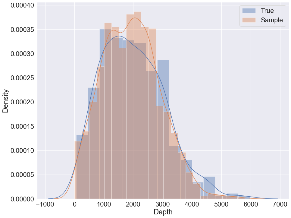
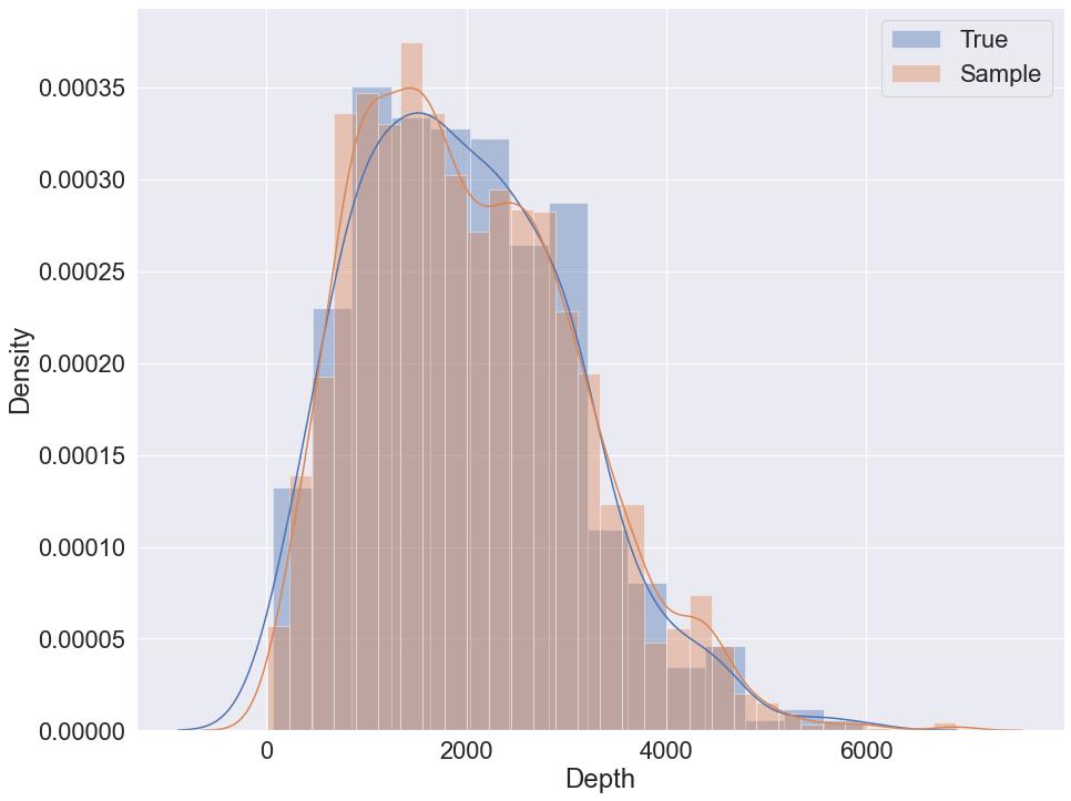
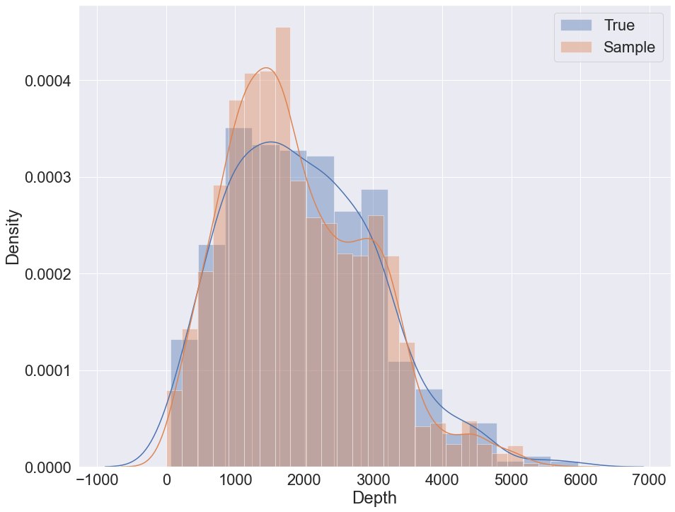
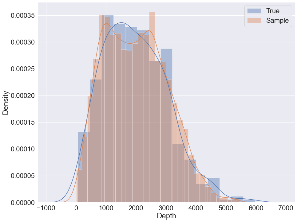
The data set contains 9 variables with 442 samples. The target variable for prediction in the following example is ‘Depth’. The variable is also used to visually evaluate sampling quality via distribution plot.
Sampling and corresponding network structure
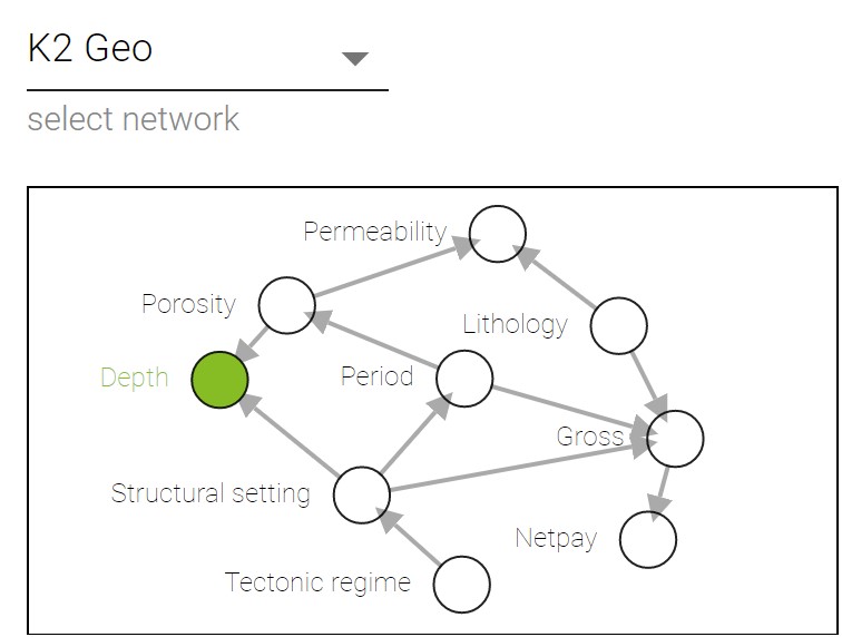
K2 metric sampling example
To sample using K2 metric the following code can be used:
train, validation = train_test_split(data, test_size=0.1)
bn = Nets.HybridBN(has_logit=False, use_mixture=False)
bn.add_nodes(info)
bn.add_edges(discretized_data,  scoring_function=('K2',K2Score))
bn.fit_parameters(train)
# prediction
val_pred = bn.predict(validation.iloc[:,:8], 5)
# sampling
sample = bn.sample(5000, parall_count=5)
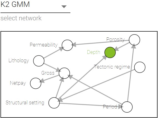
Sampling with K2 + GMM example
To sample using K2 with GMM the following code can be used:
train, validation = train_test_split(data, test_size=0.1)
bn = Nets.HybridBN(has_logit=False, use_mixture=True)
bn.add_nodes(info)
bn.add_edges(discretized_data,  scoring_function=('K2',K2Score))
bn.fit_parameters(train)
# prediction
val_pred = bn.predict(validation.iloc[:,:8], 5)
# sampling
sample = bn.sample(5000, parall_count=5)
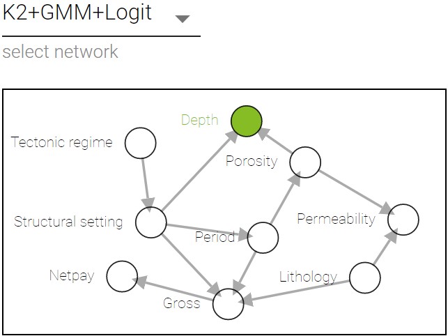
Sampling with K2 + GMM + logit nodes example
To sample using K2 with GMM and logit nodes the following code can be used:
train, validation = train_test_split(data, test_size=0.1)
bn = Nets.HybridBN(has_logit=True, use_mixture=True)
bn.add_nodes(info)
bn.add_edges(discretized_data,  scoring_function=('K2',K2Score))
bn.fit_parameters(train)
# prediction
val_pred = bn.predict(validation.iloc[:,:8], 5)
# sampling
sample = bn.sample(5000, parall_count=5)
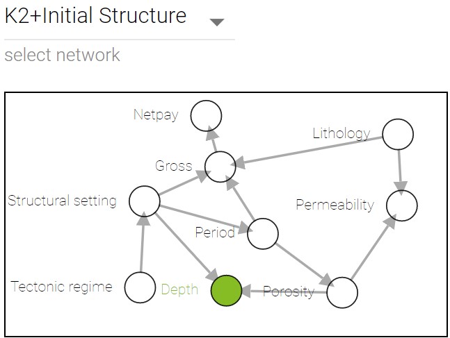
K2 with initial structure sampling
To sample using K2 and initial structure the following code can be used:
params = {'init_nodes': ['Tectonic regime', 'Period', 'Lithology', 'Structural setting', 'Gross','Netpay', 'Porosity','Permeability', 'Depth'],
    'init_edges':[('Period', 'Permeability'), ('Structural setting', 'Netpay'), ('Gross', 'Permeability')],}

train, validation = train_test_split(data, test_size=0.1)
bn = Nets.HybridBN(has_logit=True, use_mixture=True)
bn.add_nodes(info)
bn.add_edges(discretized_data,  scoring_function=('K2',K2Score), params=params)
bn.fit_parameters(train)
# prediction
val_pred = bn.predict(validation.iloc[:,:8], 5)
# sampling
sample = bn.sample(5000, parall_count=5)
Prediction MSE table for both examples
Hyperparameters combinations |
Geological data MSE |
Social data MSE |
|---|---|---|
K2 |
1014.59 |
6066.5 |
K2 + GMM |
974.35 |
5149.5 |
K2 + GMM + logit |
1018.84 |
6657.93 |
K2 + initial structure |
1056.06 |
12506.47 |
House Prices Dataset examples: Feature analysis and Data Sampling
In this example we will use house prices dataset from kaggle that contains multiple categorical and continuous features. The target variable is, obviously, the price of a house.
Feature analysis example
We will try to improve prediction results of LinearRegressor by using Bayesian Networks, with the assumption that we have a lack of samples and poor data, for example, only 40% of what we have in the original dataset.
To take a look at this example more precisely, please click here.
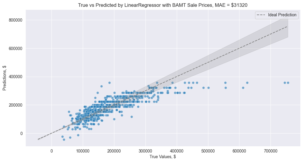
Initially, LinearRegressor cannot fit the model, that is why we get a result below
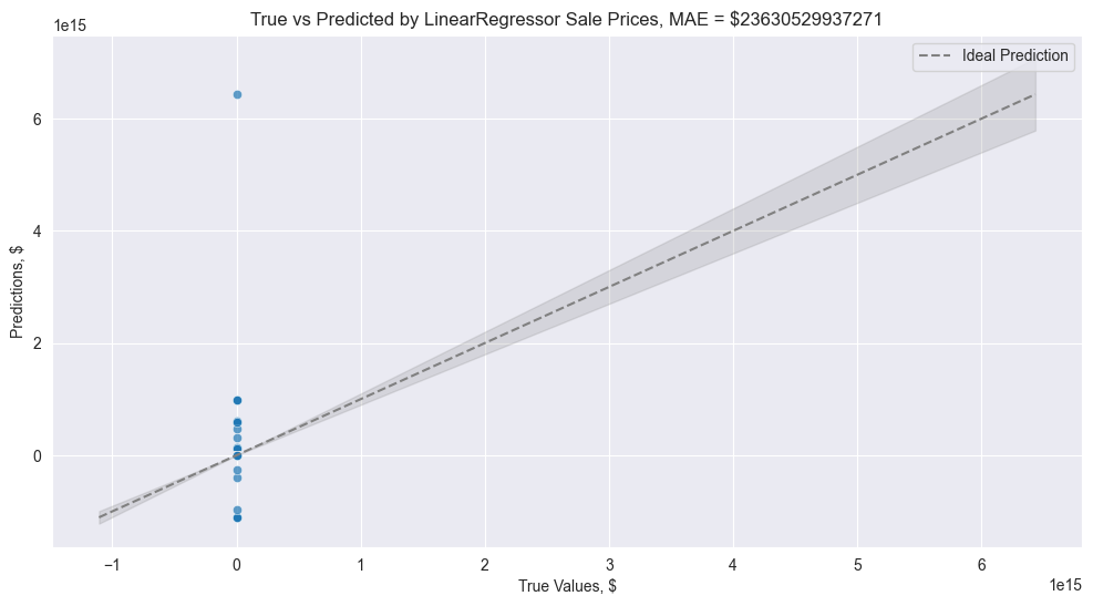
But after we learn the model only on predictors that are parent nodes of the label variable, LinearRegressor manages to provide a far better result
Synthetic data sampling example
We will try to improve prediction results of adaboost regressor by using Bayesian Networks. We will have to drop some of continuous data because BAMT has some limitations when lots of continuous columns are present, sampling will take a lot of time. We also had to drop some columns to make total number of features 20, so that the inference of BN time will be fast enough to run this example on any hardware without waiting for too long.
To take a look at this example more precisely, please click here.
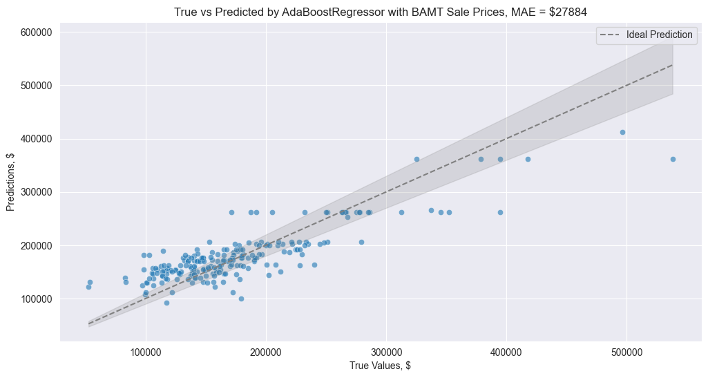
AdaBoostRegressor already has a decent result on the data
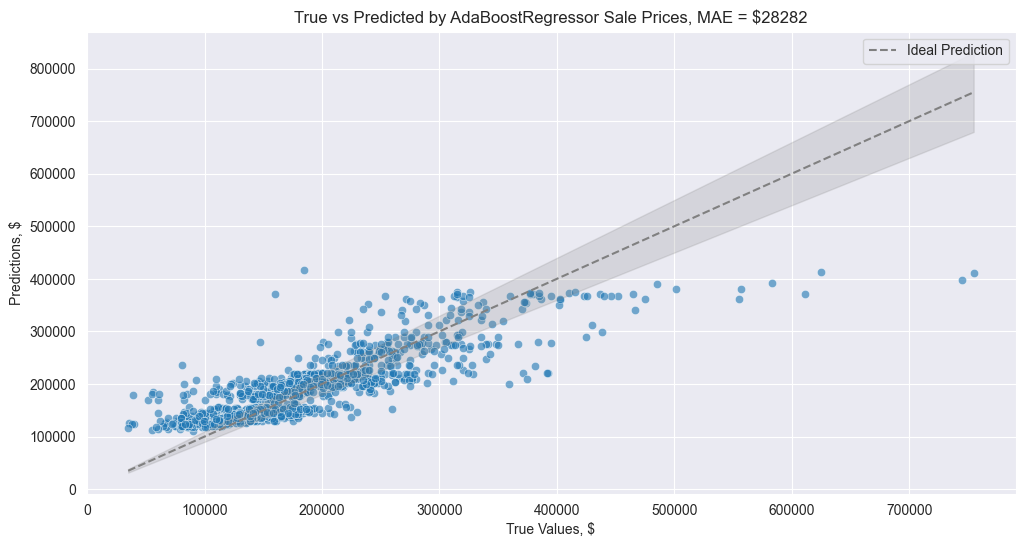
But we can improve it using synthetic data generated by BAMT
Social data example
Data Description
The second example is similar to the previous one, but carried out on different data set. Social data set consists of 30000 anonymous bank records with 9 variables each, bayesian networks were learnt on a sample with 2000 records. The target variable is ‘mean_tr’ which is mean transaction of client.
Sampling
The code used to sample from social data set is identical to the geological dataset.
K2 metric sampling example
Sampling with K2 + GMM example
Sampling with K2 + GMM + logit nodes example
K2 with initial structure sampling